Problem Introduction:
This week started off with the binary classification problem - given an image of a cat, we want to be able to tell whether it is a cat or not. We can tackle this kind of issue using a logistic regression algorithm, which is frequently implemented in neural networks.
Logistic Regression:
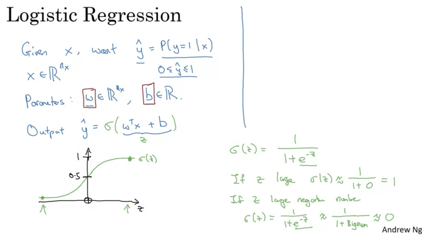
Logistic regression is a classification algorithm that is used to predict the probability of a categorical dependent variable. It is a special case of linear regression, in which the dependent variable is categorical. In logistic regression, the dependent variable is a binary variable that contains data coded as 1 (yes, success, etc.) or 0 (no, failure, etc.). In other words, the logistic regression model predicts P(Y=1) as a function of X.
If we take our image as an X-dimensional vector, and Y hat as the chance of the image being correct, W as the weights
and b as the threshold, we can calculate the probability of the image being correct by applying a sigmoid
function, as seen below in the following formula:
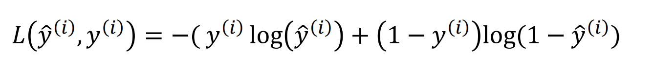
To apply this method, we first define a loss function that we want to minimise. This allows us to
measure how well we're doing on a single training sample. In this case, we define it as follows:
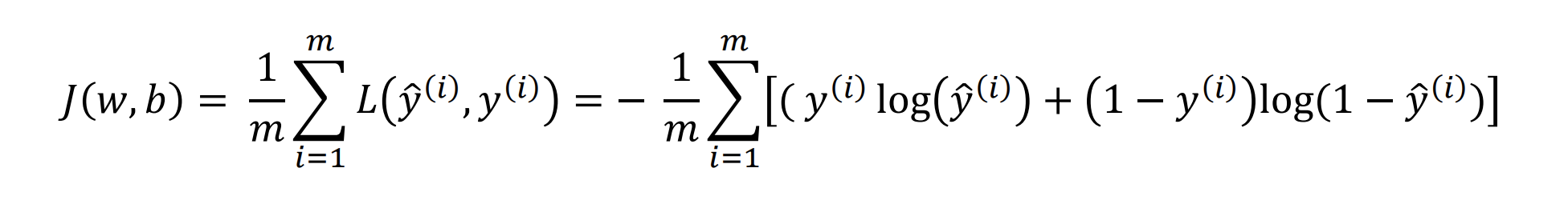
We then define the cost function as the average of the loss functions of all the training examples:
Although we now have the functions needed to calculate how well our model is doing, we still
need to define how we're going to update the weights and biases. This is where the gradient descent algorithm comes in.
Gradient Descent:
Gradient descent is an iterative algorithm that is used to find the minimum of a function. To do this, it starts at a point on a function and takes steps in the negative direction of the gradient of the function at that point. It then repeats this process until it reaches a point where the gradient is zero.
The gradient of a function is the vector of its first-order partial derivatives. The gradient points in the direction of greatest increase of the function, and its magnitude is the slope of the tangent line of the function at that point. The wonderful thing about our cost function is that it is a convex function, (i.e. it looks like a bowl), which means that it has a single global minimum.
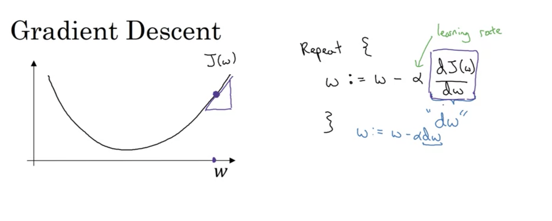
We can implement this algorithm with the following pseudocode:
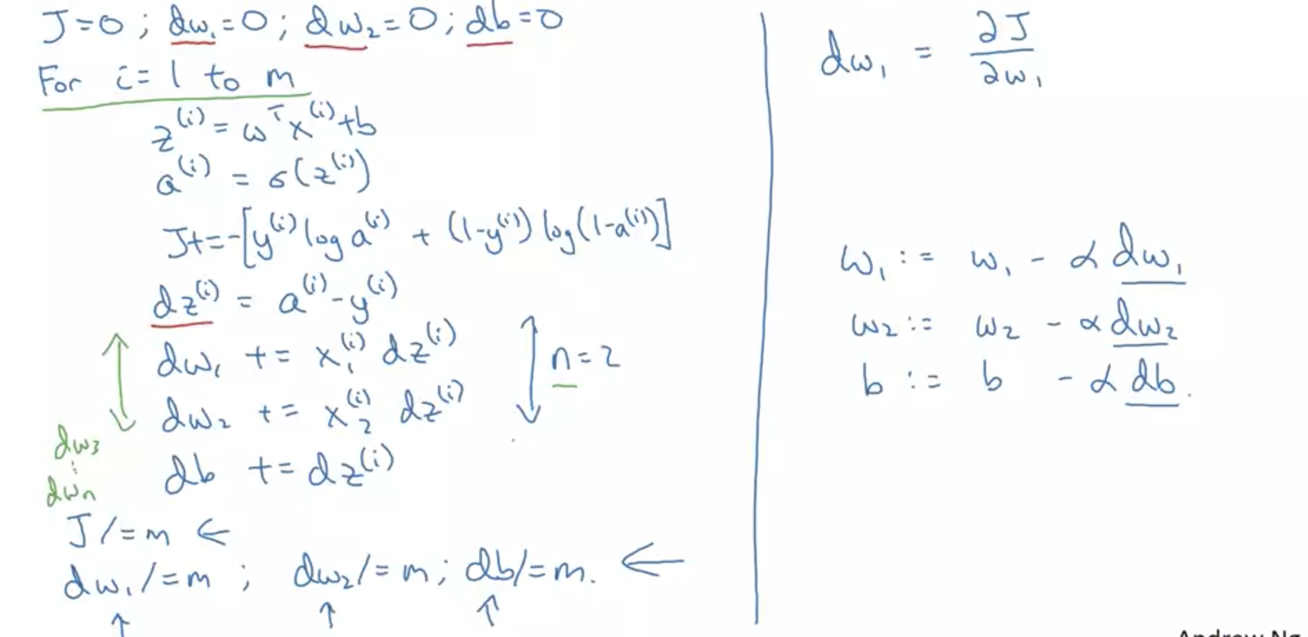
As we can see in the image above, this can lead to two sets of for loops, one for the number of iterations, and one for the number of training examples. This is because we want to update the weights and biases for each training example, and then repeat this process for the number of iterations. This can lead to a lot of computation, and so to deal with this complexity we utilise vectorization. I won't go into too much detail about how this works, but it basically allows us to perform the same operation on multiple training examples at once, which is much more efficient.
What's next?
Well, the next bit is to implement this in code, which is actually one of the assignments for this module anyway. I found trying to grasp the mathematics behind this very difficult, as it involved doing a recap of partial differentiation (something I haven't touched since A-level maths), so I diidn't actually get the time to write this code up. My aim is to try to do this for the next blogm as well as make notes on next week's topic as well. Hopefully this blog didn't bore you all too much, and I'll see you all next week!