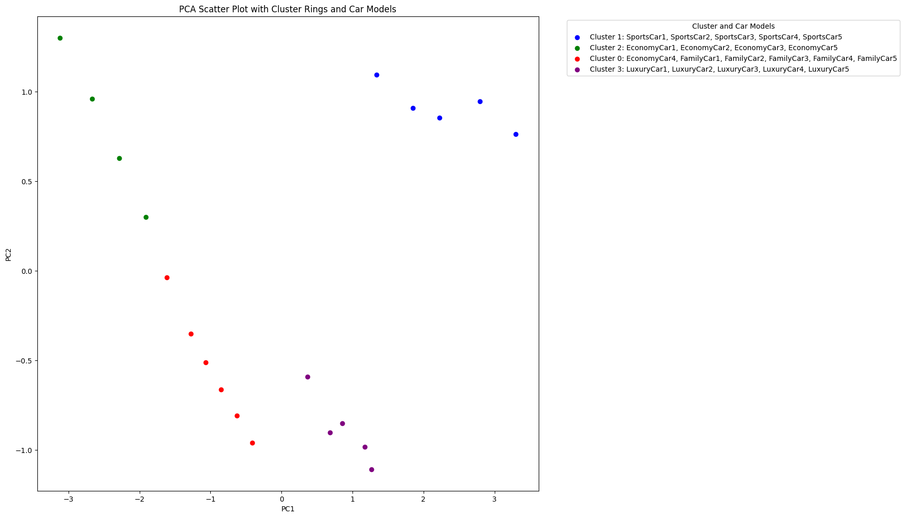
In our previous blog post, we explored how Principal Component Analysis (PCA) can be used to understand and visualize the relationships among different car models based on their features. PCA helped us identify distinct clusters and gain insights into the characteristics of each car segment. Today, we'll dive into two related techniques: Multidimensional Scaling (MDS) and Principal Coordinate Analysis (PCoA).
MDS and PCoA are similar to PCA in their goal of reducing the dimensionality of a dataset and uncovering patterns. However, while PCA focuses on correlations among samples, MDS and PCoA work with distances between samples. In this post, we'll explore how MDS and PCoA can be applied to our car dataset and compare the results with our previous PCA findings.
from ml_code.utils import load_data

# Load the dataset
data = load_data('car_data.csv')

# Print the first few rows of the dataset
data.head()

+-------------+------------+----------------+--------+--------+
|    model    | horsepower | fuel_efficiency | weight | price  |
+-------------+------------+----------------+--------+--------+
| SportsCar1  |    450     |       12       |  3500  | 150000 |
+-------------+------------+----------------+--------+--------+
| SportsCar2  |    500     |       10       |  3800  | 200000 |
+-------------+------------+----------------+--------+--------+
| SportsCar3  |    400     |       14       |  3200  | 120000 |
+-------------+------------+----------------+--------+--------+
| SportsCar4  |    480     |       11       |  3600  | 180000 |
+-------------+------------+----------------+--------+--------+
| SportsCar5  |    420     |       13       |  3400  | 140000 |
+-------------+------------+----------------+--------+--------+
Multidimensional Scaling (MDS) and Principal Coordinate Analysis (PCoA) are techniques used to visualize the level of similarity between individual cases of a dataset. They aim to create a low-dimensional representation of the data that preserves the distances between samples as much as possible. The main difference between MDS/PCoA and PCA lies in the input data. While PCA works with the original variables and their correlations, MDS and PCoA start by calculating distances between samples. These distances can be computed using various metrics, such as Euclidean distance, Manhattan distance, or even custom distance functions tailored to the specific data.
Let's apply MDS and PCoA to our car dataset and see how they help us uncover patterns and relationships among the car models. We'll use the same dataset as before, which contains information about various car models, including their horsepower, fuel efficiency, weight, and price.
First, we load the dataset and preprocess it by separating the features from the target variable (car model) and standardizing the features. Next, we calculate the distances between each pair of car models. Initially we're going to focus on Euclidean distances.
from sklearn.manifold import MDS

# Apply MDS with Euclidean distance
mds_euclidean = MDS(n_components=2, dissimilarity='euclidean', random_state=42)
X_mds_euclidean = mds_euclidean.fit_transform(X_scaled)

# Create DataFrames for MDS results
mds_euclidean_df = pd.DataFrame(data=X_mds_euclidean, columns=['MDS1', 'MDS2'])
mds_euclidean_df['Model'] = y
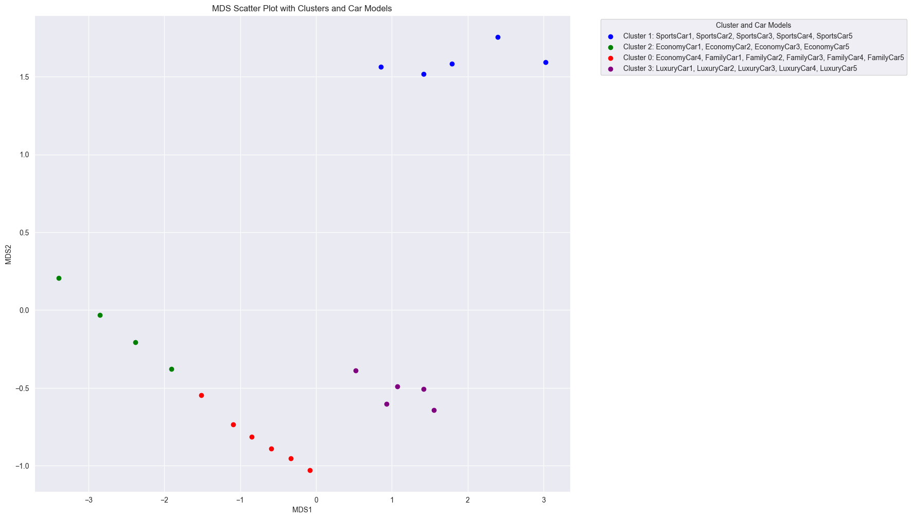
When we apply MDS using Euclidean distance as the dissimilarity metric, we obtain a scatter plot that reveals similar clustering patterns as our previous PCA analysis. The car models are grouped into distinct clusters based on their features, with sports cars, economy cars, family cars, and luxury cars forming separate clusters. In other words, clustering based on minimizing the linear distance is the same as maximizing the linear correlation.
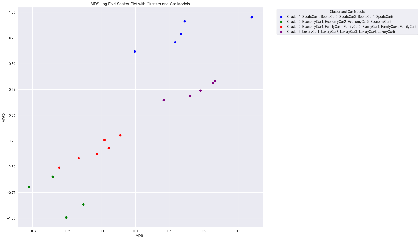
In some cases, we may want to apply MDS using a custom distance metric that captures the relative differences between samples. For example, if we used log fold change as the distance metric, we could visualize how car models differ from each other in terms of their features. This approach can be particularly useful when the absolute values of features are less important than their relative differences, eg. if we had wanted to understand how changes in say weight affected the clustering of cars.
from sklearn.metrics import pairwise_distances

# Calculate log fold change distances
X_log_fold_change = np.log1p(X) - np.log1p(X.mean())

# Apply MDS with log fold change distance
mds_log_fold_change = MDS(n_components=2, dissimilarity='precomputed', random_state=42)

# Calculate pairwise distances
distances = pairwise_distances(X_log_fold_change, metric='euclidean')

X_mds_log_fold_change = mds_log_fold_change.fit_transform(distances)

# Create DataFrames for MDS results
mds_log_fold_change_df = pd.DataFrame(data=X_mds_log_fold_change, columns=['MDS1', 'MDS2'])
mds_log_fold_change_df['Model'] = y
When we apply MDS using log fold change as the dissimilarity metric, we obtain a different perspective on the relationships between car models. The clusters themselves are the exact same, but the distances between the points are different.
In this blog post, we explored how Multidimensional Scaling (MDS) and Principal Coordinate Analysis (PCoA) can be used to uncover patterns and relationships in car data. By visualizing the distances between car models, we gained insights into the similarities and differences among different car segments. We compared the results of MDS and PCoA with our previous PCA analysis and discussed the similarities and differences between these dimensionality reduction techniques.
Both MDS / PCoA and PCA are powerful tools for exploring high-dimensional datasets and revealing underlying patterns. Both allow us to see how samples relate to each other, but they do so in different ways. PCA focuses on correlations between samples, while MDS and PCoA focus on distances. By understanding the strengths and limitations of each technique, we can choose the most appropriate method for our specific dataset and research questions.