This post took me a while to write as I wanted to make sure I understood PCA well enough. For this entire blog, I have tried to apply what I learnt by creating a custom dataset that can be used to demonstrate the power of PCA. I hope you enjoy it!
Imagine you have a dataset containing information about various car models, each with multiple features such as horsepower, fuel efficiency, weight, and price. How can you extract meaningful information from this complex data? The last thing we want to do is have to draw out each relationship between the features individually - as the number of features grows, this would become exponentially more time-consuming.
This is where Principal Component Analysis (PCA) comes to the rescue. In this blog post, we'll how it can help us understand and visualize the relationships among different car models.
Before we get our hands dirty with the car dataset, let's take a moment to grasp the concept of PCA. In simple terms, PCA is a technique that transforms a dataset with many variables into a new set of variables called principal components. These principal components are created in such a way that they capture the maximum amount of information from the original dataset while being uncorrelated with each other. Think of it as a tool that takes a complex, high-dimensional dataset and condenses it into a more manageable and interpretable form. PCA helps us identify patterns, reduce the dimensionality of the data, and visualize the relationships among the observations.
from ml_code.utils import load_data

# Load the dataset
data = load_data('car_data.csv')

# Print the first few rows of the dataset
data.head()

+-------------+------------+----------------+--------+--------+
|    model    | horsepower | fuel_efficiency | weight | price  |
+-------------+------------+----------------+--------+--------+
| SportsCar1  |    450     |       12       |  3500  | 150000 |
+-------------+------------+----------------+--------+--------+
| SportsCar2  |    500     |       10       |  3800  | 200000 |
+-------------+------------+----------------+--------+--------+
| SportsCar3  |    400     |       14       |  3200  | 120000 |
+-------------+------------+----------------+--------+--------+
| SportsCar4  |    480     |       11       |  3600  | 180000 |
+-------------+------------+----------------+--------+--------+
| SportsCar5  |    420     |       13       |  3400  | 140000 |
+-------------+------------+----------------+--------+--------+
We have information about various car models, including their horsepower, fuel efficiency, weight, and price. Our goal is to understand how these cars are related to each other based on their features.
To begin, we load the dataset into our Python environment and perform some basic preprocessing steps, such as separating the features from the target variable (car model) and standardizing the features to ensure they have zero mean and unit variance.
# Separate the features and the target variable
X = data.drop('model', axis=1)
y = data['model']

# Standardize the features
scaler = StandardScaler()
X_scaled = scaler.fit_transform(X)
Next, we apply PCA to our preprocessed dataset. In this case, we specify the number of principal components we want to keep. Since we have four features, we'll start by retaining all four components to capture the maximum amount of information. (Note: Usually in PCA, you would start with the number of components equal to the minimum of the number of observations - in this case the number of car models - or the number of features)
# Apply PCA
pca = PCA(n_components=4)
X_pca = pca.fit_transform(X_scaled)
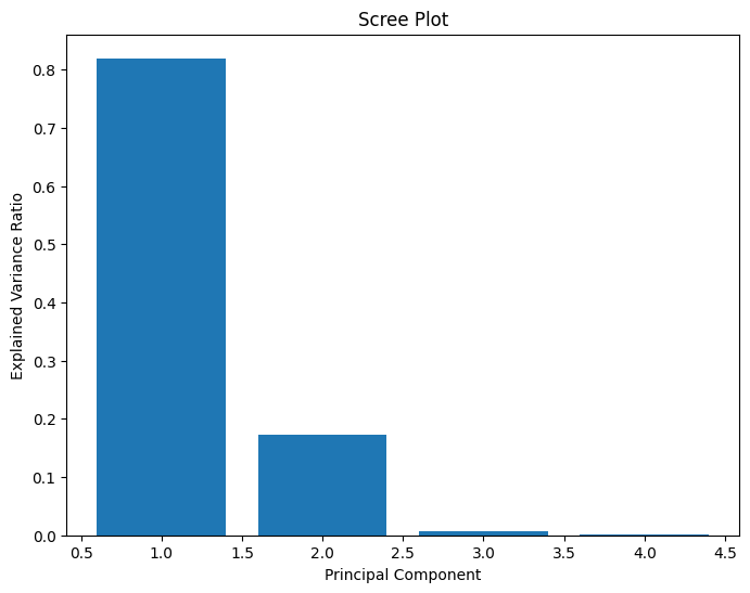
After running PCA, we obtain the transformed dataset in terms of the principal components. Each principal component is a linear combination of the original features, and they are ranked in order of the amount of variance they explain. To understand the importance of each principal component, we can examine the explained variance ratio.
print(pca.explained_variance_ratio_)

[0.81957028 0.17267014 0.00658543 0.00117415]
In our car dataset, we find the following:
This tells us that the first two principal components (PC1 and PC2) together account for a whopping 94.3% of the variance in the dataset. In other words, we can focus on these two components to gain a good understanding of the relationships among the car models.
To visualize the results, we create a scatter plot of the car models using the first two principal components (PC1 and PC2). Each point in the plot represents a car model, and we color-code them based on their category (e.g., sports cars, economy cars, family cars, luxury cars). The scatter plots reveals some fascinating insights:
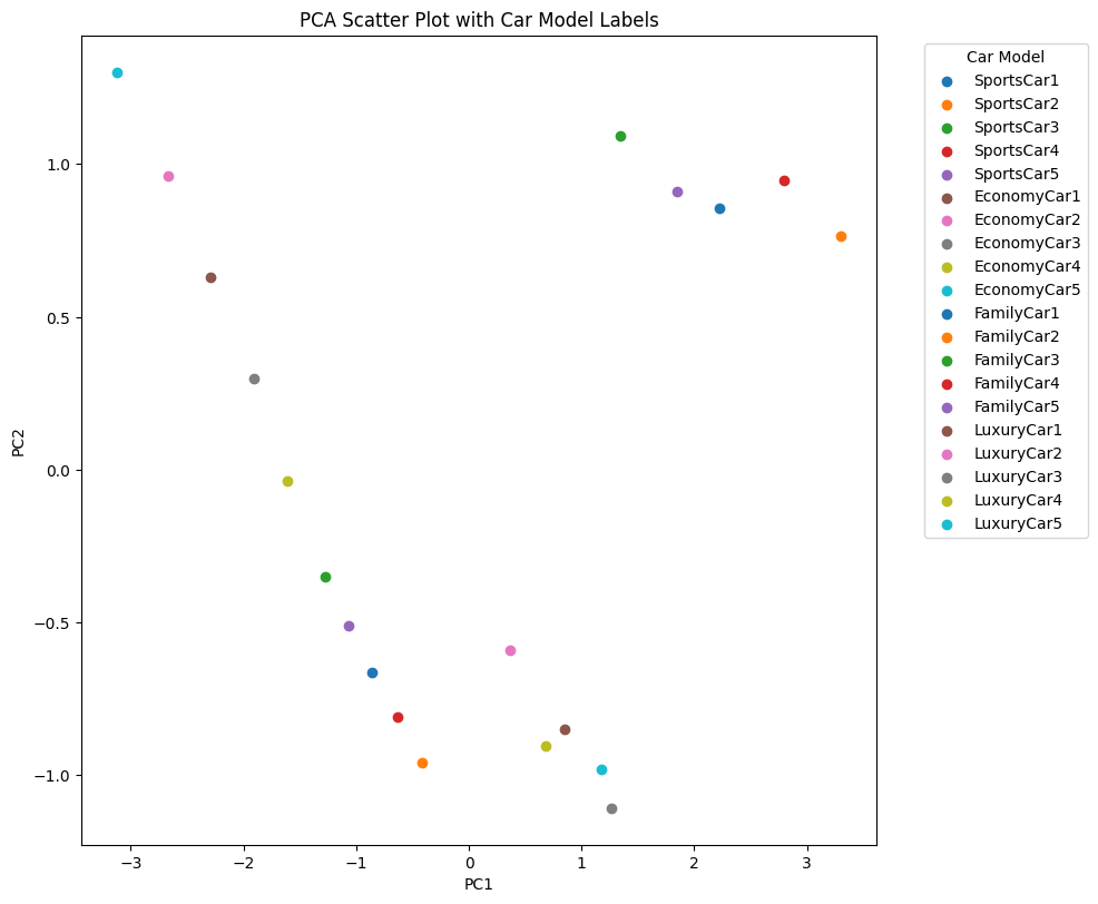
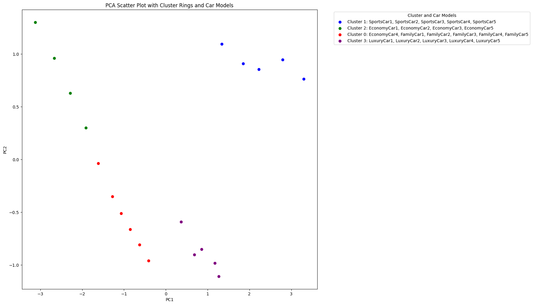
Distinct Clusters: We can clearly see four distinct clusters of car models, each representing a different category. The sports cars cluster together on the right side of the plot, while most of the economy cars form a cluster on the left side. The family cars and luxury cars occupy the middle region.
Characteristics of Clusters: The positions of the clusters along the principal components axes provide clues about their characteristics. For example, the sports cars have high positive values along PC1, indicating they likely have high horsepower, high price, and low fuel efficiency. On the other hand, the economy cars have negative values along PC1, suggesting lower horsepower, lower price, and higher fuel efficiency.
Interpretation of Principal Components: PC1 seems to capture the main differences between the car models, separating the sports cars from the economy cars. PC2 captures additional variations within the car segments, helping to differentiate the family cars from the luxury cars.
PCA has proven to be a powerful tool for exploring and understanding our car dataset. By reducing the dimensionality and visualizing the data in terms of the principal components, we gained valuable insights into the relationships among different car models.
We discovered distinct clusters representing various car categories, each with its own characteristics. The scatter plot allowed us to identify the key features that differentiate the car segments, such as performance, price, and fuel efficiency. Moreover, PCA helped us simplify the complex dataset and focus on the most important information. By retaining just the first two principal components, we were able to capture a significant portion of the variance and create an informative visualization.
In conclusion, PCA is a valuable technique for anyone dealing with high-dimensional datasets. So, the next time you encounter a dataset with numerous variables, remember the power of PCA! Apply it to your data, explore the relationships, and gain insights that can drive your analysis forward. Happy analyzing!