100 Days of ML Code - Day 8: Regularization Techniques in Machine Learning

Tuesday 21 May 2024

Introduction

In machine learning, overfitting is a common problem where a model learns the noise in the training data to the extent that it negatively impacts its performance on new, unseen data. Regularization techniques are used to prevent overfitting and improve the generalization ability of a model. In this blog post, we will explore two popular regularization methods: Ridge (L2) and Lasso (L1) regression.

Ridge (L2) Regression

Ridge regression, also known as L2 regularization, addresses the overfitting problem by adding a penalty term to the ordinary least squares objective function. The penalty term is the sum of the squared coefficients multiplied by a regularization parameter (λ). The objective function for ridge regression is:

$\sum_{i=1}^{n} (y_i - \hat{y}_i)^2 + \lambda \sum_{j=1}^{p} \beta_j^2$

where $y_i$ is the actual value, $\hat{y}_i$ is the predicted value, $\beta_j$ is the coefficient of the $j$ -th feature, and $\lambda$ is the regularization parameter. By adding this penalty term, ridge regression shrinks the coefficients towards zero, but they never reach exactly zero. This allows the model to retain all the features while reducing their impact on the predictions. The optimal value of $\lambda$ is typically determined using cross-validation techniques, such as k-fold cross-validation.

Ridge Regression with Discrete Variables

Ridge regression can also be applied to models with discrete variables. For example, when predicting the influence of diet on the size of mice, the regularization term would be the sum of the squared differences in means between the high-fat diet and the normal diet groups, multiplied by $\lambda$ .

Ridge Regression in Logistic Regression

Ridge regularization can be applied to logistic regression by adding the penalty term to the log-likelihood function. The objective function becomes:

$\sum_{i=1}^{n} \log(1 + e^{-y_i(\beta_0 + \beta_1x_{i1} + \ldots + \beta_px_{ip})}) + \lambda \sum_{j=1}^{p} \beta_j^2$

where $y_i$ is the binary target variable, $x_{ij}$ is the value of the $j$ -th feature for the $i$ -th instance, and $\beta_j$ is the coefficient of the $j$ -th feature.

Lasso (L1) Regression

Lasso regression, or L1 regularization, is similar to ridge regression but uses the absolute values of the coefficients instead of their squares in the penalty term. The objective function for lasso regression is:

$\sum_{i=1}^{n} (y_i - \hat{y}_i)^2 + \lambda \sum_{j=1}^{p} |\beta_j|$

The key difference between lasso and ridge regression is that lasso can drive some coefficients to exactly zero, effectively performing feature selection. This property makes lasso regression useful for identifying and removing irrelevant or redundant features from the model.

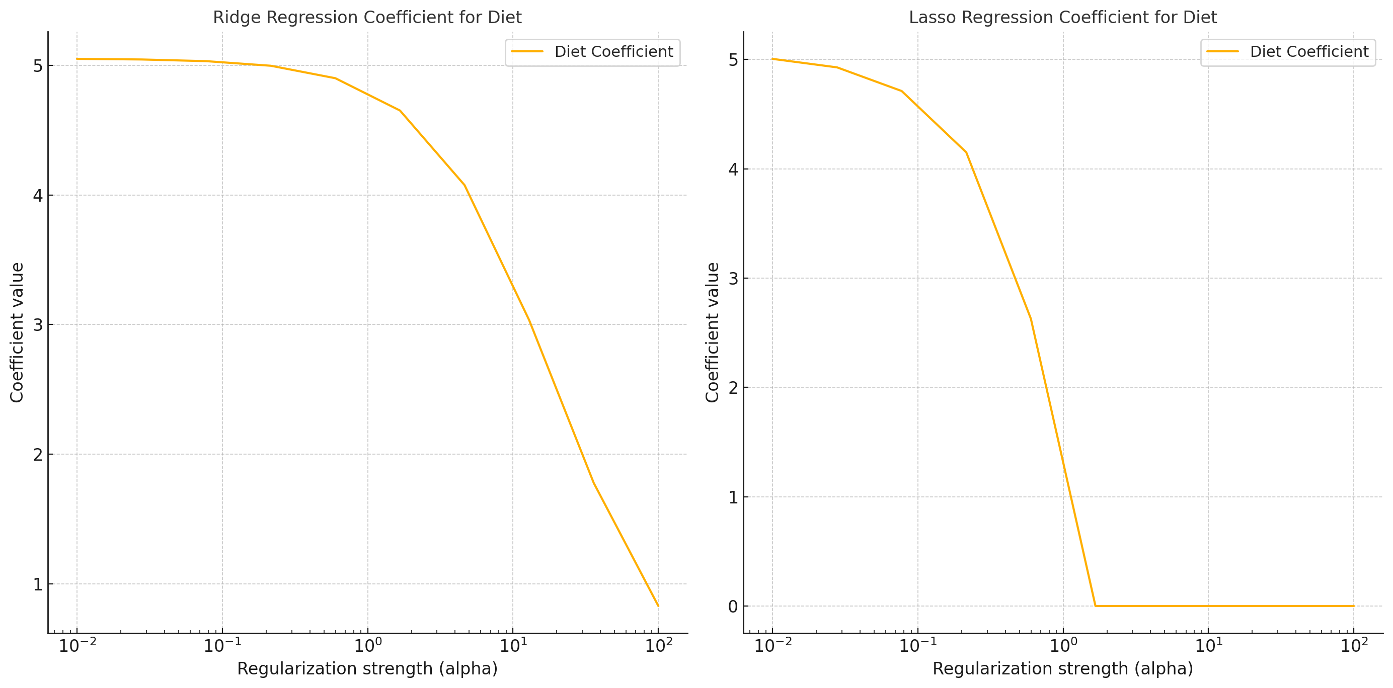
Regularisation Comparison — Regularization Comparison

Conclusion

Regularization techniques, such as ridge and lasso regression, are essential tools for preventing overfitting and improving the generalization performance of machine learning models. Ridge regression shrinks the coefficients towards zero, while lasso regression can drive some coefficients to exactly zero, performing feature selection. By understanding and applying these regularization methods, you can build more robust and interpretable models that better handle unseen data.