Continuing my journey in the 100 Days of ML Code challenge, Days 2 and 3 focus on exploring simple and multiple linear regression. These are foundational techniques in machine learning that help us understand the relationship between variables and make predictions. This post will cover the process of visualizing data, training linear regression models, making predictions, and evaluating model performance.
In Day 2, we used a simple dataset containing student scores and try to judge their correlation to the number of study hours. Our aim is to try to find a linear function that predicts a response value (score) as accurately as possible based on the feature (study hours). Let's dive into the steps involved.
The dataset used is student_scores.csv, which has two columns: "Hours" and "Scores". Our goal is to predict the "Scores" based on "Hours".
from ml_code.utils import load_data

dataset = load_data("studentscores.csv")
dataset.head()

+-------+--------+
| Hours | Scores |
+-------+--------+
|   2.5 |     21 |
|   5.1 |     47 |
|   3.2 |     27 |
|   8.5 |     75 |
|   3.5 |     30 |
+-------+--------+
First, I wanted to visualize the relationship between the number of study hours and the scores obtained. This helps us understand if there's a linear relationship between the two variables.
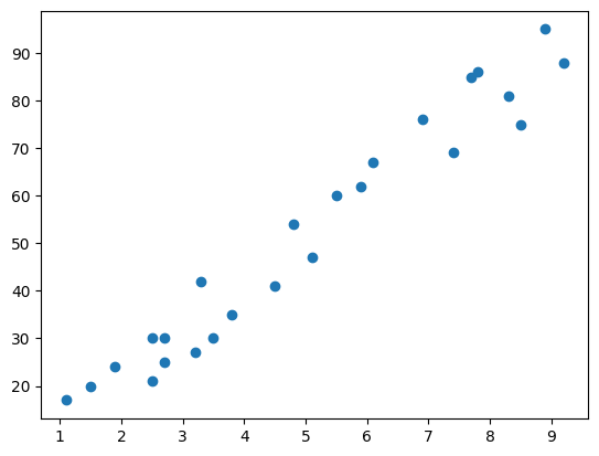
We could see a clear positive linear relationship between the nuber of study hours and the scores obtained. Therefore, it seems suitable to apply simple linear regression to this dataset.
We split the data into training and test sets, then train a simple linear regression model.
from sklearn.model_selection import train_test_split
from sklearn.linear_model import LinearRegression

features_train, features_test, labels_train, labels_test = train_test_split(features, labels, test_size=0.25, random_state=0)

regressor = LinearRegression()
regressor.fit(features_train, labels_train)
After training the model, we can make predictions on the test set and evaluate its performance by looking at metrics like Mean Absolute Error (MAE), Mean Squared Error (MSE), and Root Mean Squared Error (RMSE).
But what are these metrics? Let's break them down:
Mean Absolute Error: This metric measures the average magnitude of the errors in a set of predictions, without considering their direction. It’s the average over the test sample of the absolute differences between prediction and actual observation where all individual differences have equal weight. It gives an idea of how wrong the predictions are on average.
Mean Squared Error: This metric measures the average of the squares of the errors — that is, the average squared difference between the estimated values and the actual value. MSE is more sensitive to larger errors because the squaring of each term effectively penalizes larger errors more than smaller ones.
Root Mean Squared Error: This is the square root of the mean of the squared errors. RMSE is a good measure of how accurately the model predicts the scores. It gives an idea of how large the errors are.
labels_pred = regressor.predict(features_test)
print("Mean Absolute Error:", metrics.mean_absolute_error(labels_test, labels_pred))
print("Mean Squared Error:", metrics.mean_squared_error(labels_test, labels_pred))
print(
    "Root Mean Squared Error:",
    metrics.mean_squared_error(labels_test, labels_pred) ** 0.5,
)

Mean Absolute Error: 4.130879918502482
Mean Squared Error: 20.33292367497996
Root Mean Squared Error: 4.509204328368805
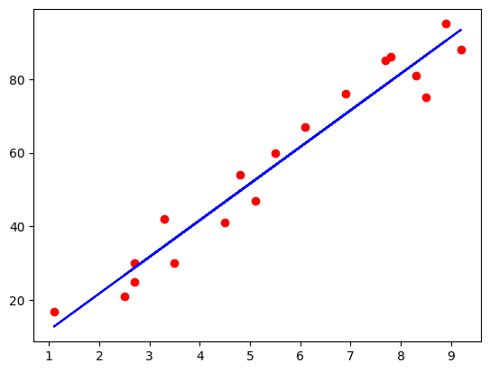
The mean absolute error value hovers around 4.13. The RMSE value of 4.51 also indicates a similar range of error in the model's predictions. Let's see if our line of best fit passes the eye test, and looks like it fits the data well.
We can see that the line of best fit closely follows the trend of the data points, indicating a good fit.
Considering the lack of complexity in the dataset, the simple linear regression model performed okay in predicting student scores based on study hours. The model is able to find the linear relationship between the two variables, but struggles sometimes with accuracy when predicting scores. This could be due to the small size of the dataset, and the fact that within the dataset, the score values are more spread out towards the higher end of the scale.
Multiple linear regression extends the concept of simple linear regression by considering multiple features to predict a response variable. The steps involved in multiple linear regression is very similar to that shown in the simple example above, but there are a few things to be mindful of that we will get into.
The dataset used for multiple linear regression is a bit more complex, containing multiple features that we can use to predict the response variable.
We are using the 50_Startups.csv dataset, which has columns like "R&D Spend", "Administration", "Marketing Spend", "State" and "Profit".
dataset = load_data("50_Startups.csv")
dataset.head()

+------------+----------------+----------------+------------+------------+
| R&D Spend  | Administration | Marketing Spend| State      | Profit     |
+------------+----------------+----------------+------------+------------+
| 165349.2   | 136897.8       | 471784.1       | New York   | 192261.83  |
| 162597.7   | 151377.59      | 443898.53      | California | 191792.06  |
| 153441.51  | 101145.55      | 407934.54      | Florida    | 191050.39  |
| 144372.41  | 118671.85      | 383199.62      | New York   | 182901.99  |
| 142107.34  | 91391.77       | 366168.42      | Florida    | 166187.94  |
+------------+----------------+----------------+------------+------------+
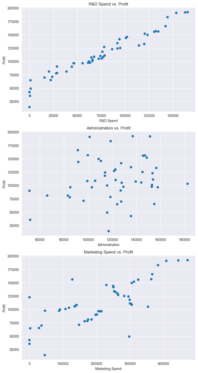
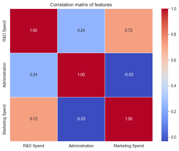
Before we can start using a linear regression model, we need to describe the current data, and check some of our assumptions. We need to make sure that there is some linearity between the features and the response variable, and that the features are not highly correlated with each other. Most of this can be done with visualisations or correlation matrices. I will spare you the code implementation here and just focus on the results.
We know that there is some categorical data in the "State" column. We will need to encode this data before we can use it in our model. We're going to do this through one-hot-encoding to convert the categorical data into numerical data. This will allow us to use the "State" column in our model. Something to keep note of here is that we want to avoid the dummy variable trap, which is where we have multiple columns that are highly correlated with each other.
eg. If we have a column for "New York" and "California", we don't need a column for "Florida" as well, as the model can infer that if the other two columns are 0, then the value must be "Florida".
After preprocessing the data, we can split it into training and test sets, and train a multiple linear regression model.
dataframe = pd.get_dummies(dataframe, columns=["State"], drop_first=True)

features = dataframe.drop("Profit", axis=1)
labels = dataframe["Profit"]

X_train, X_test, y_train, y_test = train_test_split(
    features, labels, test_size=0.2, random_state=0
)

regressor = LinearRegression()
regressor.fit(X_train, y_train)
We can now make predictions on the test set and evaluate the model's performance. With multiple linear regression, we can use the same metrics as in simple linear regression to evaluate the model's accuracy, but we also incorporate the R-squared and adjusted R-squared values to understand how well the model fits the data.
What are these metrics? Let's break them down:
R-squared: This metric measures the proportion of the variance in the dependent variable that is predictable from the independent variables. It provides an indication of the goodness of fit of the model. The higher the R-squared value, the better the model fits the data.
Adjusted R-squared: This metric adjusts the R-squared value based on the number of independent variables in the model. It provides a more accurate measure of the model's goodness of fit when there are multiple independent variables.
y_pred = regressor.predict(X_test)

r2 = metrics.r2_score(y_test, y_pred)
adjusted_r2 = 1 - (1 - r2) * (len(y_test) - 1) / (len(y_test) - X_test.shape[1] - 1)
mse = metrics.mean_squared_error(y_test, y_pred)
rmse = np.sqrt(mse)
mae = metrics.mean_absolute_error(y_test, y_pred)

print(f"R-squared value: {r2}")
print(f"Adjusted R-squared value: {adjusted_r2}")
print(f"Mean Squared Error: {mse}")
print(f"Root Mean Squared Error: {rmse}")
print(f"Mean Absolute Error: {mae}")

R-squared value: 0.9347068473282424
Adjusted R-squared value: 0.8530904064885454
Mean Squared Error: 83502864.03257754
Root Mean Squared Error: 9137.990152794953
Mean Absolute Error: 7514.293659640612
The R-squared value is quite high, indicating that the model explains a significant portion of the variance in profit. However, the Adjusted R-squared is lower, suggesting that the model may include some less relevant predictors or could be improved by refining the feature set. The MSE seems large, but the RMSE provides a clearer picture. An RMSE of 9,138 means the model's typical prediction error is around 8.16% of the average profit ($112,012.64), which may (or may not) be an acceptable level of error depending on the context this is used.