Saturday 18 May 2024

Introduction

Today we're diving into logistic regression, a fundamental classification algorithm used to predict the probability of a binary outcome. While it's called regression, logistic regression is actually used for classification tasks. In this blog post, we'll explore the logistic regression model, the sigmoid function that powers it, and the importance of gradient descent in training the model.

Understanding Logistic Regression

Logistic regression is a statistical method used to model the probability of a binary outcome based on one or more predictor variables. It is a linear model, but instead of predicting a continuous value like in linear regression, logistic regression predicts the probability of an event occurring.

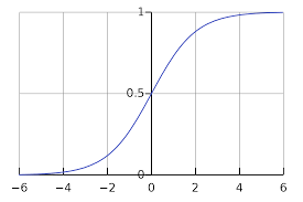
The key idea behind logistic regression is to use the logistic function, also known as the sigmoid function, to transform the linear combination of the predictor variables into a probability value between 0 and 1. The sigmoid function maps any real-valued number to a value between 0 and 1, making it suitable for representing probabilities.

The Sigmoid Function

The sigmoid function is defined as:

where $z$ is the linear combination of the predictor variables and their coefficients:

Here, $\beta_0$ is the intercept term, and $\beta_1, \beta_2, ..., \beta_n$ are the coefficients corresponding to the predictor variables $x_1, x_2, ..., x_n$.

The sigmoid function has an S-shaped curve that maps the input values to the range [0, 1]. It has the following properties:

• As $z$ approaches positive infinity, $\sigma(z)$ approaches 1.

• As $z$ approaches negative infinity, $\sigma(z)$ approaches 0.

• At $z = 0$, $\sigma(z) = 0.5$.

These properties make the sigmoid function ideal for representing the probability of a binary outcome.

The Dataset

The dataset we'll be using contains information about users in a social network. We have features like user id, gender, age, and estimated salary. A car company has just launched a brand new luxury SUV, and we want to predict which users of the social network are likely to buy this SUV. The last column is a binary column indicating whether the user bought the SUV or not.

import numpy as np
from ml_code.utils import load_data

data = load_data("Social_Network_Ads.csv")
data.head()

+-----------+--------+-----+----------------+-----------+
|  User ID  | Gender | Age | EstimatedSalary| Purchased |
+-----------+--------+-----+----------------+-----------+
| 15624510  | Male   |  19 |          19000 |         0 |
| 15810944  | Male   |  35 |          20000 |         0 |
| 15668575  | Female |  26 |          43000 |         0 |
| 15603246  | Female |  27 |          57000 |         0 |
| 15804002  | Male   |  19 |          76000 |         0 |
+-----------+--------+-----+----------------+-----------+

Preprocessing

Before training the logistic regression model, we need to preprocess the data. We'll scale the "Age" and "EstimatedSalary" features using StandardScaler from scikit-learn. This will help the model converge faster during training.

from sklearn.compose import ColumnTransformer
from sklearn.preprocessing import StandardScaler

transformer = ColumnTransformer(
    transformers=[("scaler", StandardScaler(), ["Age", "EstimatedSalary"])],
    remainder="drop",
)

features = transformer.fit_transform(data)
target = data["Purchased"]

Training the Model

We'll split the data into training and testing sets and then train a logistic regression model using scikit-learn's LogisticRegression class.

from sklearn.model_selection import train_test_split
from sklearn.linear_model import LogisticRegression

X_train, X_test, y_train, y_test = train_test_split(
    features, target, test_size=0.25, random_state=0
)

model = LogisticRegression(random_state=0)
model.fit(X_train, y_train)

The Role of Gradient Descent

Training a logistic regression model involves finding the optimal values for the coefficients $\beta_0, \beta_1, ..., \beta_n$ that maximize the likelihood of the observed data. This is typically done using an optimization algorithm called gradient descent. Gradient descent is an iterative optimization algorithm that seeks to find the minimum of a cost function. I won't bore you with the details (as there's so many resources online that will do a better job explaining it) but the gist of it is is that it works by taking steps in the direction of the steepest decrease in the cost function. This process continues until the algorithm converges to the minimum. We have to be careful with our step size when using gradient descent, as too large a step size can cause the algorithm to overshoot the minimum, while too small a step size can slow down convergence. Here's an excellent video that explains gradient descent (and logistic regression itself) in more detail:

Evaluating the Model

Let's evaluate the trained model on the test set using metrics like confusion matrix and accuracy score.

from sklearn.metrics import confusion_matrix, accuracy_score

y_pred = model.predict(X_test)
confusion_matrix(y_test, y_pred), accuracy_score(y_test, y_pred)

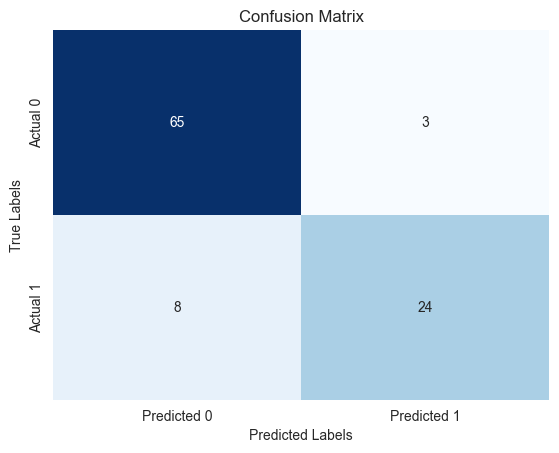
The confusion matrix shows that the model has only misclassified 11 users out of the 100 in the test set. The accuracy score of 0.89 indicates that the model has performed well in predicting whether a user will buy the SUV or not.

We can also visualize the decision boundary of the logistic regression model.

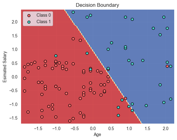
The decision boundary plot shows that the model has effectively separated the users who bought the SUV from those who didn't.

Conclusion

In this blog post, we explored logistic regression, a powerful algorithm for binary classification problems. We discussed the sigmoid function that forms the core of logistic regression and the importance of gradient descent in training the model. By applying logistic regression to a real-world dataset, we demonstrated its effectiveness in predicting whether a user will buy a product or not. This blog was relatively short, but that's because most of the time was spent understanding the mathematics behind it. I would really recommend the youtube video above if you're interested, as I found it did a great job explaining the concepts in a way that I could actually understand. I hope you enjoyed this post, and I'll see you in the next one!